Jstable 包进行亚组分析-R语言

用法：
TableSubgroupMultiGLM(
  formula,  # 模型公式，通常用于生存分析
  var_subgroups = NULL,  # 要进行分析的多个亚组变量，默认为 NULL
  var_cov = NULL,  # 额外调整的协变量，默认为 NULL
  data,  # 数据集或 survey 包中的 svydesign 设计对象
  family = "binomial",  # 模型家族，可选 "gaussian"（正态分布）、"binomial"（二项分布）、"poisson"（泊松分布）或 "quasipoisson"（准泊松分布）
  decimal.estimate = 2,  # 估计值的小数位数，默认为 2
  decimal.percent = 1,  # 百分比的小数位数，默认为 1
  decimal.pvalue = 3,  # P 值的小数位数，默认为 3
  line = FALSE  # 是否在亚组变量之间包含换行符，默认为 FALSE
)

# 安装 jstable 包（如未安装）
# install.packages("jstable")

# 加载必要的包
library(readr)
library(forestploter)
library(dplyr)
library(jstable)

# 读取 CSV 数据
dt <- read.csv("depression_survey.csv", sep = ',', header = TRUE)

# 将多个变量转换为因子
dt$Gender <- factor(dt$Gender)
dt$Education_Level <- factor(dt$Education_Level)
dt$Marital_Status <- factor(dt$Marital_Status)
dt$Depression_Status <- factor(dt$Depression_Status)
dt$Chronic_Illness <- factor(dt$Chronic_Illness)
dt$Family_History_Depression <- factor(dt$Family_History_Depression)

# 创建新的年龄分组 Age.degree
dt <- dt %>%
  mutate(Age.degree = case_when(
    Age < 40 ~ 1,
    Age >= 40 & Age < 65 ~ 2,
    Age >= 65 ~ 3
  ))

# 将 Age.degree 转换为因子
dt$Age.degree <- factor(dt$Age.degree)

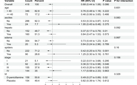
# 使用 TableSubgroupMultiGLM 进行亚组分析
res <- TableSubgroupMultiGLM(
  formula = Depression_Status ~ Weekly_Activity_Hours,  
  var_subgroups = c("Age.degree", "Gender", "Education_Level", "Marital_Status",
                    "Chronic_Illness", "Family_History_Depression"),
  data = dt,  # 指定数据集
  family = "binomial",  # 使用逻辑回归
  decimal.estimate = 2,  # 估计值保留两位小数
  decimal.pvalue = 3  # P 值保留三位小数
)

# 查看分析结果
print(res)

# 处理 P 值，将列表中的 P 值提取为数值
res$`P value` <- sapply(res$`P value`, function(x) {
  if (is.numeric(x)) {
    return(x)
  } else if (is.character(x)) {
    return(as.numeric(x))
  } else if (is.list(x)) {
    return(as.numeric(x[[1]]))
  } else {
    return(NA)
  }
})

# 保存结果为 CSV 文件
write.csv(res, 'subgroup_analysis_results.csv', row.names = FALSE)

# 定义森林图的主题
tm <- forest_theme(
  base_size = 10,       
  refline_col = "grey",
  refline_lwd = 2,
  ci_col = "#1E9C76",
  refline_lty = "solid",
  arrow_type = "closed",    
  ci_lty = 1,
  ci_Theight = 0.2,
  ci_lwd = 2.3
)

# 选择需要绘制的列
res1 <- res[, c(1:3, 9, 10, 7, 8)]

# 绘制森林图
p <- forest(
  res1,
  est = res$OR,
  lower = res$Lower,
  upper = res$Upper,
  ci_column = 5,
  xlim = c(0.9, 1.1),
  ticks_at = c(0.90, 1.00, 1.10),
  ref_line = 1,
  sizes = 0.8,
  arrow_lab = c("Low Risk", "High Risk"),
  theme = tm
)

# 保存森林图为 PNG 文件
png("subgroup_forest_plot.png", width = 3000, height = 5000, res = 300)

# 打印森林图到文件中
print(p)

# 关闭 PNG 设备，完成保存
dev.off()