python实现七大机器学习模型对比+结果分析-回归模型

#=========================================================================================
#======================================1.库的导入及全局设置================================
#=========================================================================================
import pandas as pd
import numpy as np
import matplotlib.pyplot as plt
import os
import shap
from sklearn.model_selection import train_test_split, GridSearchCV, learning_curve
from sklearn.preprocessing import StandardScaler
from sklearn.metrics import r2_score, mean_squared_error, mean_absolute_error
from scipy.stats import linregress
from sklearn.ensemble import GradientBoostingRegressor, RandomForestRegressor
from xgboost import XGBRegressor
from sklearn.svm import SVR
from sklearn.kernel_ridge import KernelRidge
from sklearn.neighbors import KNeighborsRegressor
from sklearn.neural_network import MLPRegressor
import matplotlib
matplotlib.use('TkAgg')
plt.rcParams['font.sans-serif'] = ['SimHei']
plt.rcParams['axes.unicode_minus'] = False
#=========================================================================================
#======================================2.加载数据数据预处理，设置输出路经================================
#=========================================================================================
file_path = r'C:\Users\yinzhiqiang\Desktop\修改\XGBoost_MultiClass_Output_Final\回归模拟数据.xlsx'  # 定义输入数据文件的路径
output_folder = r'C:\Users\yinzhiqiang\Desktop\修改\XGBoost_MultiClass_Output_Final\Analysis_Results_Complete'  # 定义输出结果的文件夹路径
df = pd.read_excel(file_path)  # 读取Excel文件到DataFrame
target_column = 'FVC'  # 定义目标变量（Y值）的列名
feature_columns = [col for col in df.columns if col != target_column]  # 定义特征变量（X值）的列名列表
X = df[feature_columns]  # 从DataFrame中提取所有特征列，创建特征集X
print('特征', X)
y = df[target_column]  # 从DataFrame中提取目标列，创建目标集y
print('标签', y)
# 将数据按7:3的比例划分为训练集和测试集
X_train, X_test, y_train, y_test = train_test_split(
    X, y, test_size=0.3, random_state=42
)
#标准化处理消除量纲的影响
scaler = StandardScaler().fit(X_train)
X_train_scaled = pd.DataFrame(scaler.transform(X_train), columns=X.columns, index=X_train.index)
X_test_scaled = pd.DataFrame(scaler.transform(X_test), columns=X.columns, index=X_test.index)
print(f"数据集划分完毕: 训练集({len(X_train)}), 测试集({len(X_test)})")  # 打印数据集划分结果
#=========================================================================================
#======================================3.定义模型，设置超参数================================
#=========================================================================================
models_to_run = [
    {'name': 'GBDT', 'estimator': GradientBoostingRegressor(random_state=42),
     'param_grid': {'n_estimators': [100, 200], 'learning_rate': [0.05, 0.1]}, 'needs_scaling': False},
    {'name': 'XGB', 'estimator': XGBRegressor(random_state=42, n_jobs=-1),
     'param_grid': {'n_estimators': [100, 200], 'learning_rate': [0.05, 0.1]}, 'needs_scaling': False},
    {'name': 'RF', 'estimator': RandomForestRegressor(random_state=42),
     'param_grid': {'n_estimators': [100, 200], 'min_samples_leaf': [1, 5]}, 'needs_scaling': False},
    {'name': 'KRR', 'estimator': KernelRidge(),
     'param_grid': [{'kernel': ['rbf'], 'alpha': [0.1, 1]}, {'kernel': ['linear'], 'alpha': [0.1, 1]}],
     'needs_scaling': True},
    {'name': 'SVR', 'estimator': SVR(), 'param_grid': {'C': [10, 100], 'kernel': ['rbf']}, 'needs_scaling': True},
    {'name': 'KNN', 'estimator': KNeighborsRegressor(), 'param_grid': {'n_neighbors': [5, 7], 'metric': ['minkowski']},
     'needs_scaling': True},
    {'name': 'MLP', 'estimator': MLPRegressor(random_state=42, max_iter=1000, early_stopping=True),
     'param_grid': {'hidden_layer_sizes': [(50,), (100,)], 'solver': ['adam'], 'alpha': [0.001, 0.01]},
     'needs_scaling': True}
]
#=========================================================================================
#======================================4.回归拟合散点图函数================================
#=========================================================================================
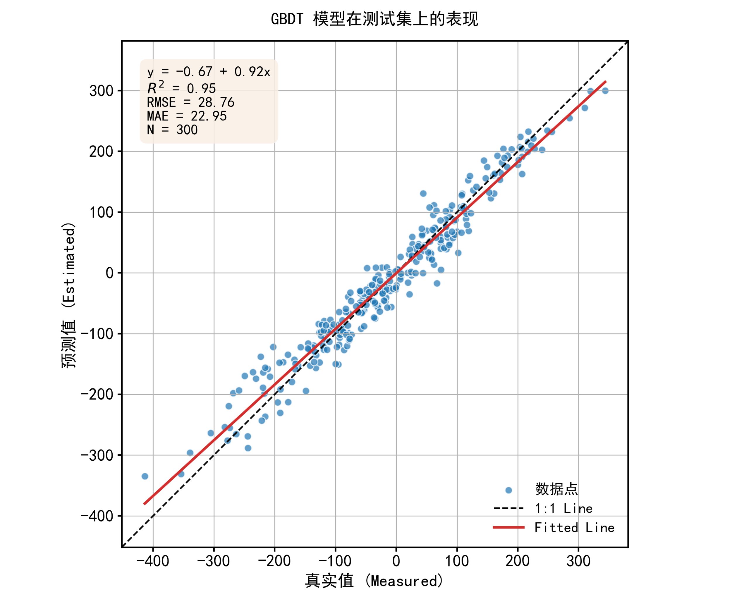
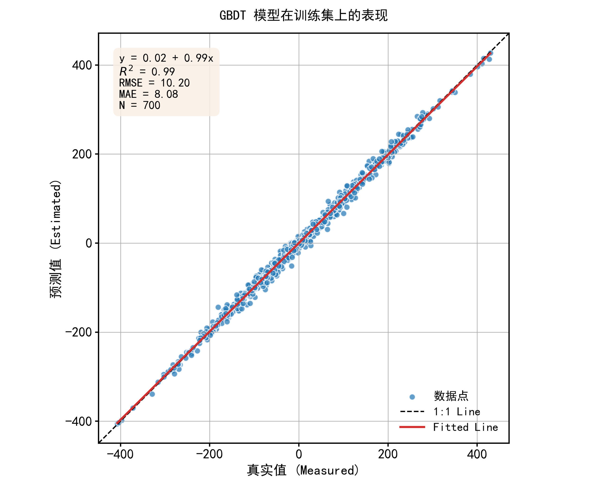
def plot_prediction_results(y_true, y_pred, title, save_path):
    fig, ax = plt.subplots(figsize=(10, 8))  # 创建一个图形和坐标轴对象
    r2 = r2_score(y_true, y_pred)  # 计算R2
    rmse = np.sqrt(mean_squared_error(y_true, y_pred))  # 计算均方根误差
    mae = mean_absolute_error(y_true, y_pred)  # 计算平均绝对误差
    n = len(y_true)  # 获取样本数量
    slope, intercept, _, _, _ = linregress(y_true, y_pred)  # 计算线性回归的斜率和截距
    # 绘制所有数据点的散点图
    ax.scatter(y_true, y_pred, c='#1f77b4', label='数据点', alpha=0.7, s=50, edgecolors='w')
    overall_min = min(y_true.min(), y_pred.min())  # 计算所有数据的最小值
    overall_max = max(y_true.max(), y_pred.max())  # 计算所有数据的最大值
    buffer = (overall_max - overall_min) * 0.05  # 计算坐标轴的缓冲范围
    plot_lim_min = overall_min - buffer  # 定义坐标轴的最小值
    plot_lim_max = overall_max + buffer  # 定义坐标轴的最大值
    ax.set_xlim(plot_lim_min, plot_lim_max)  # 设置x轴范围
    ax.set_ylim(plot_lim_min, plot_lim_max)  # 设置y轴范围
    ax.plot([plot_lim_min, plot_lim_max], [plot_lim_min, plot_lim_max],  # 绘制1:1对角线
            linestyle='--', color='black', linewidth=1.5, label='1:1 Line')
    x_fit = np.array([y_true.min(), y_true.max()])  # 创建用于绘制拟合线的数据点
    ax.plot(x_fit, slope * x_fit + intercept,  # 绘制回归拟合线
            color='#D32F2F', linewidth=2.5, label='Fitted Line')
    stats_text = (f'y = {intercept:.2f} + {slope:.2f}x\n'  # 准备要显示的统计文本
                  f'$R^2$ = {r2:.2f}\n'
                  f'RMSE = {rmse:.2f}\n'
                  f'MAE = {mae:.2f}\n'
                  f'N = {n}')
    ax.text(0.05, 0.95, stats_text, transform=ax.transAxes, fontsize=14,  # 在图上添加统计文本框
            verticalalignment='top',
            bbox=dict(boxstyle='round,pad=0.5', fc='#FAF0E6', alpha=0.85, edgecolor='none'))
    ax.set_xlabel('真实值 (Measured)', fontsize=16, fontweight='bold')  # 设置x轴标签
    ax.set_ylabel('预测值 (Estimated)', fontsize=16, fontweight='bold')  # 设置y轴标签
    ax.set_title(title, fontsize=16, fontweight='bold', pad=16)  # 设置图表标题
    legend = ax.legend(loc='lower right', frameon=False, fontsize=14)  # 显示图例
    ax.tick_params(axis='both', which='major', length=4, width=1.5, labelsize=16)  # 自定义坐标轴刻度样式
    for label in ax.get_xticklabels() + ax.get_yticklabels():  # 遍历所有刻度标签
        label.set_fontweight('bold')  # 将刻度标签设置为粗体
    for spine in ax.spines.values():  # 遍历图表的四个边框
        spine.set_linewidth(1.5)  # 设置边框粗细
    ax.grid(True)  # 显示网格线
    ax.set_aspect('equal', 'box')  # 设置坐标轴比例为1:1
    plt.tight_layout()  # 自动调整布局
    plt.savefig(save_path, dpi=300)  # 保存图表到指定路径
    print(f"图表已保存到: {save_path}")  # 打印保存路径
    plt.close(fig)  # 关闭当前图形，防止在循环中打开过多窗口

#=========================================================================================
#======================================5.残差图函数================================
#=========================================================================================
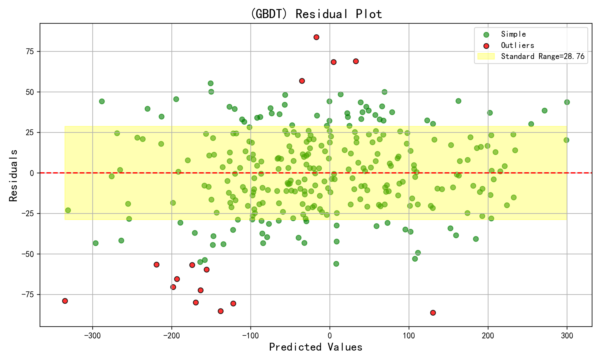
def plot_residuals(y_true, y_pred, model_name, save_path):
    residuals = y_true - y_pred  # 计算残差（真实值 - 预测值）
    std_dev = np.std(residuals)  # 计算残差的标准差
    outlier_threshold = 1.96 * std_dev  # 定义异常值阈值（约95%置信区间）
    is_outlier = np.abs(residuals) > outlier_threshold  # 创建一个布尔掩码，标记异常值
    fig, ax = plt.subplots(figsize=(10, 6))  # 创建图形和坐标轴
    ax.scatter(y_pred[~is_outlier], residuals[~is_outlier], c='green', alpha=0.6, label='Simple')  # 绘制正常值的散点（绿色）
    ax.scatter(y_pred[is_outlier], residuals[is_outlier], c='red', alpha=0.8, edgecolors='k',
               label='Outliers')  # 绘制异常值的散点（红色）
    ax.axhline(y=0, color='red', linestyle='--')  # 绘制y=0的参考线
    ax.fill_between([min(y_pred), max(y_pred)], -std_dev, std_dev,  # 绘制标准范围的阴影区域
                    color='yellow', alpha=0.3, label=f'Standard Range={std_dev:.2f}')
    ax.set_xlabel('Predicted Values', fontsize=14)  # 设置x轴标签
    ax.set_ylabel('Residuals', fontsize=14)  # 设置y轴标签
    ax.set_title(f'({model_name}) Residual Plot', fontsize=16)  # 设置图表标题
    ax.legend()  # 显示图例
    ax.grid(True)  # 显示网格线
    plt.tight_layout()  # 自动调整布局
    plt.savefig(save_path, dpi=300)  # 保存图表
    plt.close(fig)
#=========================================================================================
#======================================6.shap摘要图函数================================
#=========================================================================================
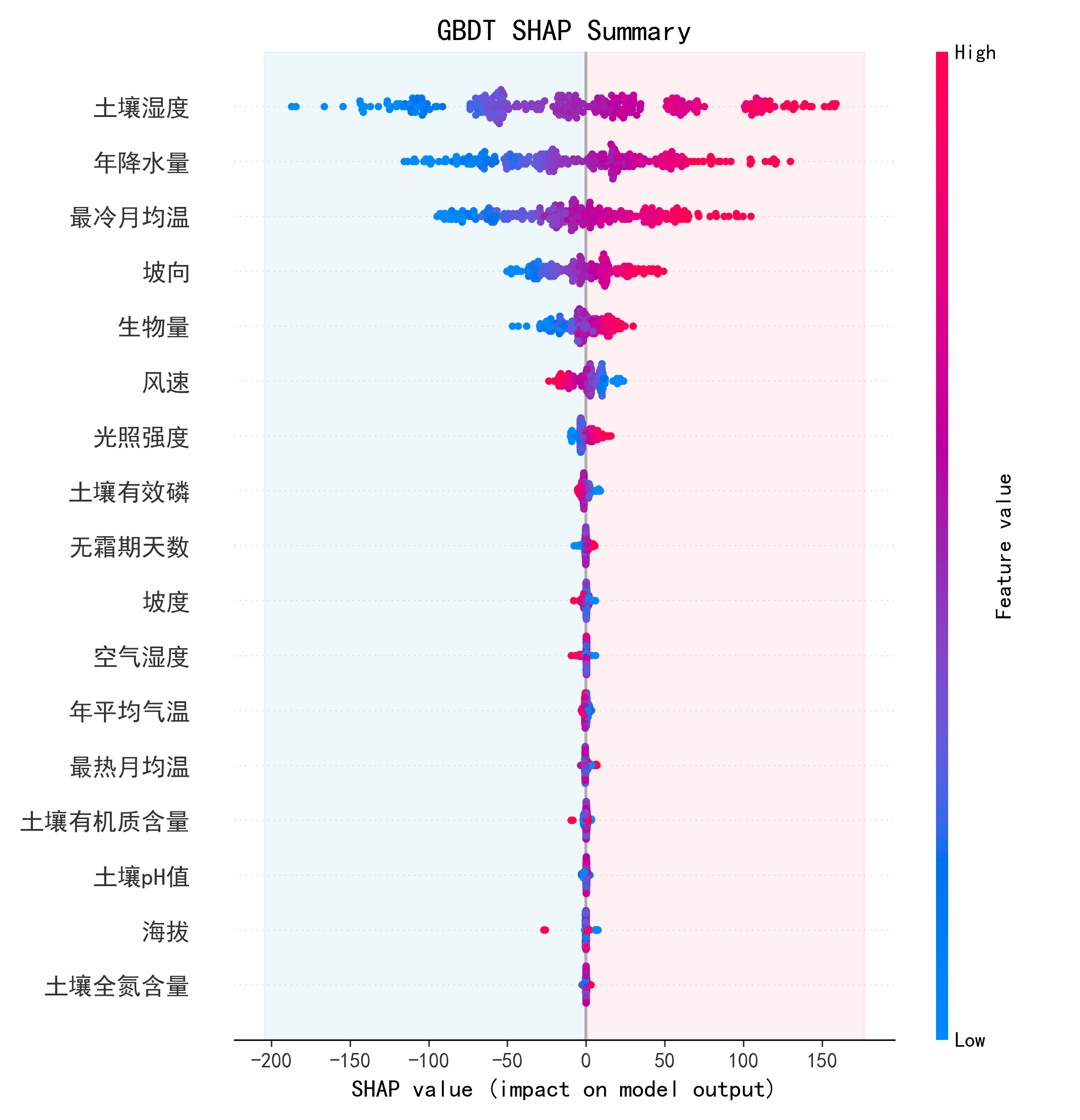
def plot_shap_summary(model, X, feature_names, model_name, save_path):
    print(f"正在为 {model_name} 进行 SHAP 分析")
    if any(s in str(type(model)).lower() for s in ['gradient', 'randomforest', 'xgb']):  # 判断是否为树模型
        explainer = shap.TreeExplainer(model)  # 如果是，使用高效的TreeExplainer
    else:  # 否则为其他模型
        if not hasattr(model, 'predict'):  # 检查模型是否有predict方法
            # 为 SVR 等没有 predict 方法但有 decision_function 的模型添加 predict
            model.predict = lambda x: model.decision_function(x)
        X_summary = shap.sample(X, 100, random_state=42)  # 从数据中抽样作为背景数据，以加速KernelExplainer
        explainer = shap.KernelExplainer(model.predict, X_summary)  # 使用通用的KernelExplainer
    shap_values = explainer.shap_values(X)  # 计算SHAP值
    shap.summary_plot(shap_values, X, feature_names=feature_names, show=False)  # 生成SHAP摘要图，但不立即显示
    ax = plt.gca()  # 获取当前的坐标轴对象
    ax.axvspan(ax.get_xlim()[0], 0, color='lightblue', alpha=0.2, zorder=0)  # 在SHAP值小于0的区域添加浅蓝色背景
    ax.axvspan(0, ax.get_xlim()[1], color='lightpink', alpha=0.2, zorder=0)  # 在SHAP值大于0的区域添加浅粉色背景
    plt.title(f'{model_name} SHAP Summary', fontsize=16)  # 设置图表标题
    fig = plt.gcf()  # 获取当前的图形对象
    fig.tight_layout()  # 自动调整布局
    fig.savefig(save_path, dpi=300)
    print(f"SHAP 图表已保存到: {save_path}")
    plt.close(fig)
#=========================================================================================
#======================================7.学习曲线胡子hi函数================================
#=========================================================================================
def plot_all_learning_curves(all_curves_data, save_path):
    plt.figure(figsize=(12, 10))  # 创建一个图形
    colors = matplotlib.colormaps['tab10']  #获取颜色映射
    min_score, max_score = 1.0, -2.0  # 初始化Y轴范围的最小和最大值
    for i, (model_name, train_sizes, train_scores, test_scores) in enumerate(all_curves_data):  # 遍历每个模型的数据
        test_scores_mean = np.mean(test_scores, axis=1)  # 计算交叉验证得分的平均值
        if test_scores_mean.min() < min_score: min_score = test_scores_mean.min()  # 更新Y轴最小值
        if test_scores_mean.max() > max_score: max_score = test_scores_mean.max()  # 更新Y轴最大值
        train_scores_mean = np.mean(train_scores, axis=1)  # 计算训练得分的平均值
        train_scores_std = np.std(train_scores, axis=1)  # 计算训练得分的标准差
        test_scores_std = np.std(test_scores, axis=1)  # 计算交叉验证得分的标准差
        plt.plot(train_sizes, train_scores_mean, 'o-', color=colors(i),  # 绘制训练得分曲线
                 label=f'{model_name} Training')
        plt.fill_between(train_sizes, train_scores_mean - train_scores_std,  # 绘制训练得分的标准差范围
                         train_scores_mean + train_scores_std, alpha=0.1, color=colors(i))
        plt.plot(train_sizes, test_scores_mean, 's-', color=colors(i), alpha=0.7,  # 绘制交叉验证得分曲线
                 label=f'{model_name} Cross-validation')
        plt.fill_between(train_sizes, test_scores_mean - test_scores_std,  # 绘制交叉验证得分的标准差范围
                         test_scores_mean + test_scores_std, alpha=0.1, color=colors(i))
    plt.title('Learning Curves for All Models', fontsize=18)  # 设置标题
    plt.xlabel('Training examples', fontsize=14)  # 设置x轴标签
    plt.ylabel('$R^2$', fontsize=14)  # 设置y轴标签
    padding = (max_score - min_score) * 0.1  # 计算Y轴的缓冲范围
    y_min = min_score - padding  # 确定Y轴最小值
    y_max = min(1.05, max_score + padding)  # 确定Y轴最大值，但不超过1.05
    plt.ylim(y_min, y_max)  # 设置Y轴范围
    plt.legend(loc="best")  # 显示图例
    plt.grid(True)  # 显示网格线
    plt.tight_layout()  # 自动调整布局
    plt.savefig(save_path, dpi=300)
    print(f"\n所有模型的学习曲线对比图已保存到: {save_path}")
    plt.close('all')
#=========================================================================================
#=====================================8.主循环调用绘图函数================================
#=========================================================================================
all_learning_curves_data = []  # 初始化一个列表，用于存储所有模型的学习曲线数据
for model_config in models_to_run:  # 开始遍历 `models_to_run` 列表中的每一个模型配置
    model_name = model_config['name']  # 获取模型名称
    estimator = model_config['estimator']  # 获取模型估算器实例
    param_grid = model_config['param_grid']  # 获取超参数网格
    print(f"开始处理模型: {model_name}")
    X_train_to_use, X_test_to_use = X_train_scaled, X_test_scaled  # 使用标准化后的数据
    print(f"\n开始为 {model_name} 进行超参数搜索...")
    grid_search = GridSearchCV(estimator=estimator, param_grid=param_grid, cv=5, scoring='r2', n_jobs=-1,verbose=1)  # 配置网格搜索对象
    grid_search.fit(X_train_to_use, y_train)  # 在训练数据上执行网格搜索
    print(f"找到的最佳参数组合: {grid_search.best_params_}")  # 打印找到的最佳超参数
    print(f"在交叉验证中得到的最佳 R² 分数: {grid_search.best_score_:.4f}")  # 打印最佳交叉验证分数
    best_model = grid_search.best_estimator_  # 获取经过优化的最佳模型实例

    y_train_pred = best_model.predict(X_train_to_use)  # 在训练集上进行预测
    y_test_pred = best_model.predict(X_test_to_use)  # 在测试集上进行预测
    plot_prediction_results(y_train, y_train_pred, f'{model_name} 模型在训练集上的表现',  # 绘制训练集预测结果图
                            os.path.join(output_folder, f'{model_name}_performance_TRAIN.png'))
    plot_prediction_results(y_test, y_test_pred, f'{model_name} 模型在测试集上的表现',  # 绘制测试集预测结果图
                            os.path.join(output_folder, f'{model_name}_performance_TEST.png'))
    plot_residuals(y_test, y_test_pred, model_name, os.path.join(output_folder, f'{model_name}_residuals.png'))  # 绘制残差图
    plot_shap_summary(best_model, X_test_to_use, feature_names=X_test.columns, model_name=model_name,  # 绘制SHAP摘要图
                      save_path=os.path.join(output_folder, f'{model_name}_shap_summary.png'))
    train_sizes, train_scores, test_scores = learning_curve(  # 调用sklearn的学习曲线函数
        estimator=best_model, X=X_train_to_use, y=y_train,  # 传入模型和训练集
        cv=5, n_jobs=-1, train_sizes=np.linspace(0.1, 1.0, 5), scoring="r2"  # 配置交叉验证、并行数、训练集大小划分和评分标准
    )
    all_learning_curves_data.append((model_name, train_sizes, train_scores, test_scores))  # 将计算结果存入列表
plot_all_learning_curves(all_learning_curves_data,os.path.join(output_folder, 'ALL_MODELS_learning_curves.png'))  # 调用函数绘制所有模型的学习曲线
print(f"所有结果图表已保存至: {output_folder}")